37 min to read
Machine Learning Summary
Recording and Learning
目录
介绍
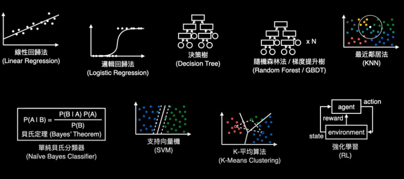
经典算法
线性回归(Linear Regression) 支持向量机(Support Vector Machine, SVM) k-近邻(K-Nearest Neighbors, KNN) 逻辑回归(Logistic Regression) 决策树(Decision Tree) k-平均(k-means) 随机森林(Random Forest) 朴素贝叶斯(Naive Bayes)
损失函数
交叉熵 & KL散度(Cross Entropy & KL Divergence) 最大似然估计(Maximum Likelihood Estimation, MLE) & 最大后验估计(Maximum A Posteriori Estimation, MAP)
激活函数
Softmax Sigmoid Tanh Relu ELU GELU
其它
介绍
机器学习算法大致可以分为以下三类:
监督学习算法(Supervised Algorithms):在监督学习训练过程中,可以由训练数据集学到或建立一个模式(函数 / learning model),并依此模式推测新的实例。通过已标注的数据(输入-输出对)学习映射关系,用于预测或分类。如,线性回归、逻辑回归、决策树、支持向量机。
无监督学习算法 (Unsupervised Algorithms):这类算法从无标注数据中发现隐藏模式或结构,没有特定的目标输出,一般将数据集分为不同的组。如,K均值聚类、层次聚类、主成分分析、自编码器。
强化学习算法 (Reinforcement Algorithms):通过与环境的交互学习最优策略,以最大化长期奖励。算法根据输出结果(决策)的成功或错误来训练自己,通过大量经验训练优化后的算法将能够给出较好的预测。类似有机体在环境给予的奖励或惩罚的刺激下,逐步形成对刺激的预期,产生能获得最大利益的习惯性行为。如,Q-Learning、深度Q网络(DQN)、策略梯度(Policy Gradient)。
线性回归
一、定义与核心思想
一种用于建模连续变量之间关系的监督学习算法。其核心假设是目标变量与特征之间存在线性关系,并通过拟合最佳直线(或超平面)进行预测,使得预测值与真实值之间的误差最小。其又分为两种类型,即只有一个自变量的简单线性回归(simple linear regression)与至少两组以上自变量的多变量回归(multiple regression)。
二、目标
找到最优的权重 $w$ 和偏置 $b$,使得预测值与真实值之间的均方误差(MSE)最小化。
三、详细内容
推荐看这篇知乎专栏。
四、实现流程
- 初始化模型参数(权重w和偏置b),通常设为0或小的随机值
- 计算预测值并计算损失函数(通常使用均方误差MSE)
- 计算损失函数对参数的梯度
- 使用梯度下降法更新参数
五、代码实现
import numpy as np
from sklearn.model_selection import train_test_split
from sklearn.preprocessing import StandardScaler
from sklearn.metrics import r2_score

class LinearRegression:
    def __init__(self, learning_rate=0.01, n_iterations=1000):
        """
        Initialize Linear Regression model

        Parameters:
        learning_rate -- step size for parameter updates (default 0.01)
        n_iterations -- number of training iterations (default 1000)
        """
        self.learning_rate = learning_rate
        self.n_iterations = n_iterations
        self.weights = None  # weight parameters
        self.bias = None     # bias parameter
        self.loss_history = []  # to record loss at each iteration

    def fit(self, X, y):
        """
        Train the linear regression model

        Parameters:
        X -- feature matrix of shape (n_samples, n_features)
        y -- target vector of shape (n_samples,)
        """
        n_samples, n_features = X.shape

        # 1. Initialize parameters
        self.weights = np.zeros(n_features)  # initialize weights to 0
        self.bias = 0                       # initialize bias to 0

        # 2. Gradient descent iterations
        for _ in range(self.n_iterations):
            # Forward pass: compute predictions
            y_pred = np.dot(X, self.weights) + self.bias

            # Compute loss (mean squared error)
            loss = (1 / (2 * n_samples)) * np.sum((y_pred - y) ** 2)
            self.loss_history.append(loss)

            # Compute gradients
            dw = (1 / n_samples) * np.dot(X.T, (y_pred - y))  # weight gradients
            db = (1 / n_samples) * np.sum(y_pred - y)         # bias gradient

            # Update parameters
            self.weights -= self.learning_rate * dw
            self.bias -= self.learning_rate * db

    def predict(self, X):
        """
        Make predictions using the trained model

        Parameters:
        X -- feature matrix of shape (n_samples, n_features)

        Returns:
        y_pred -- predicted values of shape (n_samples,)
        """
        return np.dot(X, self.weights) + self.bias
六、面经
Q:线性回归的基本假设有哪些?
线性关系假设(自变量X与因变量y之间存在线性关系),误差项独立同分布(无自相关),误差项之间无相关性(尤其时间序列数据),误差项正态分布(残差应服从均值为0的正态分布)
Q:如何判断线性回归模型的好坏?
R²分数来解释模型的方差解释能力(0-1,越接近1越好),均方误差(MSE)/均方根误差(RMSE)越小越好,残差分析(检查残差是否随机分布),也可以对比训练集和测试集表现来判断过拟合。
Q:什么是R²分数?
是评估线性回归模型拟合优度的指标,表示模型能够解释的目标变量方差比例。其取值范围通常在0到1之间,数值越大表示模型解释能力越强。R²通过比较模型预测误差(实际值与模型预测值的差异平方和)和基准误差(实际值与均值的差异平方和)来计算,具体来说计算公式为:R² = 1 - (模型预测误差 / 基准误差)
支持向量机
一、定义与核心思想
支持向量机是一种强大的监督学习算法,主要用于分类任务,也可用于回归(称为支持向量回归,SVR)。对于线性可分的数据集来说,这样的超平面有无穷多个(即感知机),但是几何间隔最大的分离超平面却是唯一的。SVM还包括核技巧,即对于输入空间中的非线性分类问题,可以通过非线性变换将它转化为某个维特征空间中的线性分类问题,在高维特征空间中学习线性支持向量机,这使它成为实质上的非线性分类器。SVM的的学习策略就是间隔最大化,可形式化为一个求解凸二次规划的问题。总的来说,其核心思想是寻找一个最优超平面,最大化不同类别数据之间的边界(间隔),从而提升模型的泛化能力。
二、目标
- 最大化分类间隔,即找到使间隔最大的超平面,提高模型的泛化能力。
- 最小化分类错误(在软间隔 SVM 中,允许少量样本违反间隔约束)。
三、详细内容
该知乎专栏提供了极为详细的数学推导,这个知乎专栏则更为通俗易懂。
四、实现流程
- 构造最优化问题,求解出最优化的所有α
- 计算参数 $w$ 和 $b$
- 得出超平面与决策函数
五、代码实现
from sklearn import datasets
from sklearn.model_selection import train_test_split
from sklearn.svm import SVC
from sklearn.metrics import accuracy_score

# 加载数据集
iris = datasets.load_iris()
X = iris.data
y = iris.target

# 划分训练集和测试集
X_train, X_test, y_train, y_test = train_test_split(X, y, test_size=0.3, random_state=42)

# 创建SVM分类器
clf = SVC(kernel='linear')

# 训练模型
clf.fit(X_train, y_train)

# 预测
y_pred = clf.predict(X_test)

# 计算准确率
accuracy = accuracy_score(y_test, y_pred)
print(f"Accuracy: {accuracy}")
六、面经
Q:SVM为什么追求”最大间隔”?
最大间隔能提高模型的泛化能力,使决策边界对噪声和数据扰动更鲁棒。间隔越大,未来新数据被分类错误的可能性越小。
Q:SVM的优点是什么?
(1)在高维空间中表现优秀:训练好的模型的算法复杂度是由支持向量的个数决定的,而不是由数据的维度决定的,所以SVM也不太容易产生overfitting (2)核技巧灵活,能适应复杂非线性问题:通过核函数,SVM可以隐式地将数据映射到更高维空间,从而解决线性不可分问题 (3)依赖支持向量而非全部数据,内存效率高:训练完成后,可以丢弃非支持向量的样本,节省存储空间,适合资源受限的场景
Q:SVM的缺点是什么?
(1)对参数和核函数选择敏感:惩罚系数 $C$ 控制模型对分类错误的容忍度,越大说明越不能容忍出现误差,容易过拟合;越小则越容易欠拟合。另外不同的核函数对结果影响很大,需要交叉验证调整 (2)黑盒性较强,可解释性差:相比逻辑回归能分析权重和决策树能可视化规则,SVM的决策过程较难解释,且无法直接输出概率(需额外校准,如Platt Scaling)。
Q:SVM为什么追求”最大间隔”?
最大间隔能提高模型的泛化能力,使决策边界对噪声和数据扰动更鲁棒。间隔越大,未来新数据被分类错误的可能性越小。
Q:SVM如何进行概率预测?
可以使用 Platt Scaling 进行校准,在SVM的输出(决策函数值)上训练一个逻辑回归模型,将其映射到 [0,1] 区间。
k-近邻
定义与核心思想
K-近邻 是一种基于样本的监督学习算法,可用于分类和回归任务。它的核心思想是:相似的数据点在特征空间中距离较近,因此新样本的类别或值可以由其最近的K个邻居决定。具体来说是给定一个训练数据集,对新的输入样本,在训练数据集中找到与该实例最邻近的K个样本,这K个样本的多数属于某个类,就把该输入样本呢分类到这个类中。(少数服从多数)
目标
- 分类任务:基于K个最近邻的多数投票,预测新样本的类别。
- 回归任务:基于K个最近邻的平均值,预测新样本的连续值。
详细内容
推荐看这篇文章。
实现流程
- 距离计算:对于待分类的样本点,计算它与训练集中每个样本点的距离
- 选择最近邻:根据计算的距离,选择距离最近的k个训练样本,即k-近邻名字的由来
- 投票决策:对于分类问题统计k个最近邻中各类别的数量,将待分类样本归为数量最多的类别;对于回归问题:取k个最近邻的目标值的平均值作为预测值
代码实现
import numpy as np
from collections import Counter
from sklearn.datasets import load_iris
from sklearn.model_selection import train_test_split
from sklearn.preprocessing import StandardScaler
from sklearn.metrics import accuracy_score

class KNN:
    """
    K-Nearest Neighbors classifier manual implementation

    Parameters:
        k: int, optional (default=5), number of nearest neighbors to consider
    """

    def __init__(self, k=5):
        self.k = k

    def fit(self, X, y):
        """
        Train the KNN model (actually just stores the data as KNN is a lazy learner)

        Parameters:
            X: Training feature data, array of shape [n_samples, n_features]
            y: Training target values, array of shape [n_samples]
        """
        # Standardize data (improves KNN performance)
        self.scaler = StandardScaler()
        self.X_train = self.scaler.fit_transform(X)
        self.y_train = y

    def predict(self, X):
        """
        Make predictions for test data

        Parameters:
            X: Test feature data, array of shape [n_samples, n_features]

        Returns:
            Predictions, array of shape [n_samples]
        """
        # Standardize test data (using mean and variance from training data)
        X = self.scaler.transform(X)
        # Initialize prediction array
        predictions = np.zeros(X.shape[0], dtype=self.y_train.dtype)

        # Make prediction for each test sample
        for i, x in enumerate(X):
            # 1. Calculate distances between current test sample and all training samples
            distances = self._compute_distances(x)

            # 2. Get indices of k nearest neighbors
            k_indices = np.argpartition(distances, self.k)[:self.k]

            # 3. Get labels of these k neighbors
            k_nearest_labels = self.y_train[k_indices]

            # 4. Vote for prediction (take most common class)
            most_common = Counter(k_nearest_labels).most_common(1)
            predictions[i] = most_common[0][0]

        return predictions

    def _compute_distances(self, x):
        """
        Calculate distances between one sample and all training samples (Euclidean distance)

        Parameters:
            x: Single sample point, array of shape [n_features]

        Returns:
            Array of distances, array of shape [n_train_samples]
        """
        # Euclidean distance calculation: sqrt(sum((x1 - x2)^2))
        distances = np.sqrt(np.sum((self.X_train - x) ** 2, axis=1))
        return distances
面经
Q: 如何选择合适的K值?
通过交叉验证(一种评估机器学习模型泛化能力的统计方法,核心思想是通过多次划分训练集和验证集,减少模型评估的随机性,从而更准确地估计模型在未知数据上的表现)尝试不同K值,选择在验证集上表现最好的K
Q:讲一下KNN的优点
(1)简单直观,易于实现:直接通过距离计算找到最近的邻居,无需复杂的数学推导 (2)无需训练阶段:KNN仅存储训练数据,预测时才计算距离,无需显式训练参数 (3)对数据分布没有假设:不像线性回归假设数据线性可分,或高斯朴素贝叶斯假设特征符合正态分布。KNN通过局部邻居投票,能捕捉非线性关系
Q:讲一下KNN的缺点
(1)计算复杂度高:需保存全部训练数据,内存占用大,对新样本需计算与所有训练样本的距离,时间复杂度为O(N·d) (2)高维数据效果差(维度灾难):在高维空间中,所有样本的距离趋于相似(欧氏距离区分度下降),导致邻居失去意义 (3)对不平衡数据敏感:若某类样本占90%,K个邻居中大概率全是多数类,少数类易被忽略 (4)需要特征缩放:若特征尺度差异大(如年龄[0-100]和工资[0-100000]),工资会主导距离计算
逻辑回归
一、定义与核心思想
逻辑回归是一种典型的监督学习算法,模型从带有标签的训练数据中学习规律,并对新数据进行预测。虽然被称为回归,但其实际上是分类模型,并常用于二分类。本质是假设数据服从某个分布,然后使用极大似然估计做参数的估计。其核心思想则是通过线性模型预测概率并用逻辑函数(Sigmoid函数)将线性结果映射到[0,1]区间。
二、目标
逻辑回归的目标是找到一组模型参数(权重$𝑤$和偏置$𝑏$),使得模型的预测概率尽可能接近真实的类别标签。这一目标通过最大化似然函数(或最小化损失函数)来实现。
三、详细内容
推荐看这篇文章。
四、实现流程
就是用交叉熵(最大似然估计和交叉熵在逻辑回归中是等价的)作为损失函数梯度下降训练一个感知机然后求softmax概率
五、代码实现
import numpy as np
from sklearn.preprocessing import StandardScaler

class LogisticRegression:
    """
    A manually implemented Logistic Regression class
    """

    def __init__(self, learning_rate=0.01, n_iterations=1000, fit_intercept=True, verbose=False):
        """
        Initialize the Logistic Regression model

        Parameters:
        learning_rate -- Step size for gradient descent (default: 0.01)
        n_iterations -- Number of iterations for gradient descent (default: 1000)
        fit_intercept -- Whether to add an intercept term (default: True)
        verbose -- Whether to print training progress (default: False)
        """
        self.learning_rate = learning_rate
        self.n_iterations = n_iterations
        self.fit_intercept = fit_intercept
        self.verbose = verbose
        self.weights = None
        self.scaler = StandardScaler()  # For feature standardization

    def __add_intercept(self, X):
        """
        Add intercept term (column of 1's) to feature matrix

        Parameters:
        X -- Input feature matrix (n_samples, n_features)

        Returns:
        Feature matrix with intercept term added (n_samples, n_features + 1)
        """
        intercept = np.ones((X.shape[0], 1))
        return np.concatenate((intercept, X), axis=1)

    def __sigmoid(self, z):
        """
        Sigmoid activation function mapping input to (0,1) interval

        Parameters:
        z -- Linear combination of inputs and weights

        Returns:
        Probability after sigmoid transformation
        """
        return 1 / (1 + np.exp(-z))

    def __loss(self, h, y):
        """
        Compute the logistic loss (log loss/cross-entropy loss)

        Parameters:
        h -- Predicted probabilities (n_samples,)
        y -- True labels (n_samples,)

        Returns:
        Current loss value
        """
        return (-y * np.log(h) - (1 - y) * np.log(1 - h)).mean()

    def fit(self, X, y):
        """
        Train the logistic regression model

        Parameters:
        X -- Training feature matrix (n_samples, n_features)
        y -- Training label vector (n_samples,)
        """
        # Standardize features
        X = self.scaler.fit_transform(X)

        # Add intercept term
        if self.fit_intercept:
            X = self.__add_intercept(X)

        # Initialize weights (zeros)
        self.weights = np.zeros(X.shape[1])

        # Gradient descent
        for i in range(self.n_iterations):
            # Linear combination of inputs and weights
            z = np.dot(X, self.weights)

            # Apply sigmoid to get probabilities
            h = self.__sigmoid(z)

            # Compute gradient (X.T * (h - y)) / n_samples
            gradient = np.dot(X.T, (h - y)) / y.size

            # Update weights
            self.weights -= self.learning_rate * gradient

            # Print training progress if verbose
            if self.verbose and i % 100 == 0:
                loss = self.__loss(h, y)
                print(f'Iteration {i}, Loss: {loss}')

    def predict_prob(self, X):
        """
        Predict probability of positive class

        Parameters:
        X -- Input feature matrix (n_samples, n_features)

        Returns:
        Probability of positive class (n_samples,)
        """
        # Standardize features
        X = self.scaler.transform(X)

        # Add intercept term
        if self.fit_intercept:
            X = self.__add_intercept(X)

        # Compute probabilities
        return self.__sigmoid(np.dot(X, self.weights))

    def predict(self, X, threshold=0.5):
        """
        Predict class labels

        Parameters:
        X -- Input feature matrix (n_samples, n_features)
        threshold -- Classification threshold (default: 0.5)

        Returns:
        Predicted class labels (n_samples,)
        """
        return self.predict_prob(X) >= threshold
六、面经
Q:逻辑回归和感知机的区别。
简单的感知机其实和逻辑回归类似,都是数据乘上一个回归系数矩阵 $w$ 得到一个数 $y$,不过感知机不求概率,一般会选取一个分类边界,可能 $y>0$ 就是 $A$ 类别,$y<0$ 就是 $B$ 类别。逻辑回归的损失函数由最大似然推导而来,用交叉熵损失,力图使预测概率分布与真实概率分布接近。感知机的损失函数可能有多种方法核心是针对误分类点到超平面的距离总和进行建模,即使预测的结果与真实结果误差更小,是去求得分类超平面(函数拟合)。这是两者最最根本的差异。
Q:为什么逻辑回归用交叉熵损失而不用MSE?
逻辑回归通过最大似然估计优化模型参数,而对数似然的负数就是交叉熵,因此两者本质相同。另外交叉熵是凸函数,梯度更新更高效,而MSE在逻辑回归中会导致非凸优化和梯度消失问题。
决策树
一、定义与核心思想
决策树是一种基于树结构的监督学习算法,主要用于分类和回归任务。它通过一系列规则对数据进行分割,构建一个树形模型,其中每个内部节点代表一个特征或属性上的判断条件,每个分支代表判断条件的可能结果,而每个叶节点代表一个类别(分类树)或一个具体值(回归树)。核心思想是递归地选择最优特征进行数据划分,使得划分后的子集尽可能”纯净”,即同一类别的样本尽可能集中。
二、目标
决策树的目标是构建一个泛化能力强、解释性好的模型,具体包括:
- 分类任务:叶节点表示类别标签,目标是最大化分类准确性。
- 回归任务:叶节点表示连续值,目标是最小化预测误差(如均方误差)。
此外,决策树追求:
- 局部最优性:每次划分选择当前最优特征,而非全局最优。
- 可解释性:通过树形结构直观展示决策逻辑(类似”if-then”规则)。
三、详细内容
四、实现流程
- 选择最优特征进行数据划分,常用准则有:ID3算法(信息增益),C4.5算法(信息增益比),CART算法(基尼指数)
- 从根节点开始,递归地对每个节点执行以下内容:1.选择当前最优特征作为划分标准;2.根据特征取值将数据集划分为若干子集;3.为每个子集创建子节点。(停止条件:1.当前节点所有样本属于同一类别;2.没有剩余特征可用于划分;3.样本数量小于预定阈值)
- 决策树剪枝(防止过拟合):预剪枝(在生成过程中提前停止树的生长),后剪枝(先生成完整树,再自底向上剪枝
五、代码实现
import numpy as np
from math import log
from collections import Counter

class DecisionTree:
    """
    A decision tree classifier using ID3 algorithm.

    Attributes:
        tree (dict): The constructed decision tree.
        max_depth (int): Maximum depth of the tree.
        min_samples_split (int): Minimum number of samples required to split a node.
    """

    def __init__(self, max_depth=None, min_samples_split=2):
        """
        Initialize the decision tree.

        Args:
            max_depth (int, optional): Maximum depth of the tree. Defaults to None.
            min_samples_split (int, optional): Minimum samples to split. Defaults to 2.
        """
        self.tree = {}
        self.max_depth = max_depth
        self.min_samples_split = min_samples_split

    def fit(self, X, y, depth=0):
        """
        Build the decision tree from training data.

        Args:
            X (numpy.ndarray): Feature matrix of shape (n_samples, n_features).
            y (numpy.ndarray): Target vector of shape (n_samples,).
            depth (int, optional): Current depth of the tree. Defaults to 0.

        Returns:
            dict: The constructed decision tree.
        """
        n_samples, n_features = X.shape
        n_classes = len(np.unique(y))

        # Stopping criteria
        if (n_classes == 1 or
            n_samples < self.min_samples_split or
            (self.max_depth is not None and depth == self.max_depth)):
            return self._most_common_label(y)

        # Find the best split
        best_feature, best_threshold = self._best_split(X, y, n_features)

        # If no split improves purity, return leaf node
        if best_feature is None:
            return self._most_common_label(y)

        # Split the dataset
        left_indices = X[:, best_feature] <= best_threshold
        right_indices = X[:, best_feature] > best_threshold

        # Recursively build left and right subtrees
        left_subtree = self.fit(X[left_indices], y[left_indices], depth+1)
        right_subtree = self.fit(X[right_indices], y[right_indices], depth+1)

        # Return the decision node
        return {
            'feature_index': best_feature,
            'threshold': best_threshold,
            'left': left_subtree,
            'right': right_subtree
        }

    def _best_split(self, X, y, n_features):
        """
        Find the best feature and threshold to split on.

        Args:
            X (numpy.ndarray): Feature matrix.
            y (numpy.ndarray): Target vector.
            n_features (int): Number of features.

        Returns:
            tuple: (best_feature_index, best_threshold)
        """
        best_gain = -1
        best_feature, best_threshold = None, None

        for feature_idx in range(n_features):
            thresholds = np.unique(X[:, feature_idx])
            for threshold in thresholds:
                gain = self._information_gain(X, y, feature_idx, threshold)

                if gain > best_gain:
                    best_gain = gain
                    best_feature = feature_idx
                    best_threshold = threshold

        return best_feature, best_threshold

    def _information_gain(self, X, y, feature_idx, threshold):
        """
        Calculate information gain from splitting on a feature and threshold.

        Args:
            X (numpy.ndarray): Feature matrix.
            y (numpy.ndarray): Target vector.
            feature_idx (int): Index of feature to split on.
            threshold (float): Threshold value for the split.

        Returns:
            float: Information gain.
        """
        # Parent entropy
        parent_entropy = self._entropy(y)

        # Split data
        left_indices = X[:, feature_idx] <= threshold
        right_indices = X[:, feature_idx] > threshold

        if len(y[left_indices]) == 0 or len(y[right_indices]) == 0:
            return 0

        # Calculate weighted child entropy
        n = len(y)
        n_left, n_right = len(y[left_indices]), len(y[right_indices])
        child_entropy = (n_left/n) * self._entropy(y[left_indices]) + \
                        (n_right/n) * self._entropy(y[right_indices])

        # Information gain is difference in entropy
        return parent_entropy - child_entropy

    def _entropy(self, y):
        """
        Calculate entropy of a target vector.

        Args:
            y (numpy.ndarray): Target vector.

        Returns:
            float: Entropy value.
        """
        counts = np.bincount(y)
        probabilities = counts / len(y)
        return -np.sum([p * np.log2(p) for p in probabilities if p > 0])

    def _most_common_label(self, y):
        """
        Find the most common label in a target vector.

        Args:
            y (numpy.ndarray): Target vector.

        Returns:
            int: The most common class label.
        """
        counter = Counter(y)
        return counter.most_common(1)[0][0]

    def predict(self, X):
        """
        Predict class labels for samples in X.

        Args:
            X (numpy.ndarray): Feature matrix of shape (n_samples, n_features).

        Returns:
            numpy.ndarray: Predicted class labels.
        """
        return np.array([self._predict_single(x, self.tree) for x in X])

    def _predict_single(self, x, tree):
        """
        Predict class for a single sample by traversing the tree.

        Args:
            x (numpy.ndarray): Single sample features.
            tree (dict): Decision tree or subtree.

        Returns:
            int: Predicted class label.
        """
        if not isinstance(tree, dict):
            return tree

        feature_idx = tree['feature_index']
        threshold = tree['threshold']

        if x[feature_idx] <= threshold:
            return self._predict_single(x, tree['left'])
        else:
            return self._predict_single(x, tree['right'])
六、面经
Q:简单解释决策树是如何工作的?
决策树像一棵倒置的树,关键在于”分层提问”和”逐步划分数据”。从根节点开始,根据数据的特征(如年龄、收入)一步步提问,每个节点是一个判断条件,分支是可能的答案,最终到达叶子节点得到预测结果。
Q:什么是信息增益?如何用它选择分裂特征?
信息增益衡量一个特征对分类的帮助有多大。比如”学历”特征如果能将客户明显分为”买/不买”两组,它的信息增益就高。决策树会优先选择信息增益高的特征分裂,因为能更干净地划分数据。
Q:如何防止决策树过拟合?
(1)剪枝:提前停止树的生长(限制深度)或事后剪掉不重要的分支 (2)限制参数:比如设置叶节点的最小样本数(避免用极少数样本做决策)
Q:决策树相比线性模型的优势?
(1)可解释性强:规则类似于人类决策过程 (2)无需复杂预处理:对缺失值、非线性关系更鲁棒。 (3)处理混合特征:同时处理数字、类别特征。
Q:决策树的缺点是什么?
(1)容易过拟合:可能记住噪声数据 (2)不稳定:数据微小变化可能导致树结构完全不同 (3)不擅长全局关系:比如线性关系,线性模型更加直接
k-平均
一、定义与核心思想
k-means 是一种经典的无监督学习聚类算法,用于将数据集划分为 k 个互不重叠的簇(clusters)。其目标是通过迭代优化,将数据点分配到最近的簇中心(质心),使得簇内数据点的相似性较高,而不同簇之间的差异性较大。
二、目标
k-means 的核心目标是将数据集划分为 k 个簇(clusters),使得每个数据点属于距离最近的簇中心。通过反复调整簇中心的位置,k-means 不断优化簇内的紧密度,从而获得尽量紧凑、彼此分离的簇。这可以用簇内平方误差(Within-Cluster Sum of Squares, WCSS)来度量:
$\text{WCSS} = \sum_{i=1}^{K} \sum_{\mathbf{x} \in C_i} |\mathbf{x} - \mathbf{\mu}_i|^2$
- $K$: 预设的簇数量。
- $C_i$: 第 $i$ 个簇的集合。
- $\mathbf{\mu}_i$: 第 $i$ 个簇的质心(均值向量)。
- $\mathbf{x}$: 数据点。
三、详细内容
推荐看这篇知乎专栏。
四、实现流程
- 初始化阶段:选择要聚类的数量 K,并随机选择 K 个数据点作为初始聚类中心(质心)
- 迭代阶段:对于每个数据点,计算其与所有质心的距离,将其分配到距离最近的质心所在的簇,然后对于每个簇,重新计算其质心(即该簇中所有数据点的均值),重复上述步骤,直到满足停止条件
- 停止条件:质心的位置变化小于某个阈值、达到预设的最大迭代次数或簇的分配不再改变
五、代码实现
import numpy as np
import matplotlib.pyplot as plt
from sklearn.datasets import make_blobs

class KMeans:
    """
    K-means clustering algorithm implementation

    Parameters:
    -----------
    n_clusters: int
        Number of clusters to form
    max_iter: int
        Maximum number of iterations
    tol: float
        Tolerance to declare convergence (if centroids move less than tol)
    random_state: int
        Seed for random initialization
    """

    def __init__(self, n_clusters=3, max_iter=100, tol=1e-4, random_state=42):
        self.n_clusters = n_clusters
        self.max_iter = max_iter
        self.tol = tol
        self.random_state = random_state
        self.centroids = None
        self.labels = None

    def _initialize_centroids(self, X):
        """Randomly initialize centroids by selecting K points from dataset"""
        np.random.seed(self.random_state)
        random_idx = np.random.permutation(X.shape[0])
        centroids = X[random_idx[:self.n_clusters]]
        return centroids

    def _compute_distances(self, X, centroids):
        """
        Compute distances between each data point and each centroid

        Parameters:
        -----------
        X: ndarray of shape (n_samples, n_features)
            Input data
        centroids: ndarray of shape (n_clusters, n_features)
            Current centroids

        Returns:
        --------
        distances: ndarray of shape (n_samples, n_clusters)
            Distance from each point to each centroid
        """
        distances = np.zeros((X.shape[0], self.n_clusters))
        for k in range(self.n_clusters):
            # Compute Euclidean distance (L2 norm)
            distances[:, k] = np.linalg.norm(X - centroids[k], axis=1)
        return distances

    def _assign_clusters(self, distances):
        """
        Assign each data point to the nearest centroid

        Parameters:
        -----------
        distances: ndarray of shape (n_samples, n_clusters)
            Distance from each point to each centroid

        Returns:
        --------
        labels: ndarray of shape (n_samples,)
            Cluster index for each data point
        """
        return np.argmin(distances, axis=1)

    def _update_centroids(self, X, labels):
        """
        Update centroids as the mean of data points in each cluster

        Parameters:
        -----------
        X: ndarray of shape (n_samples, n_features)
            Input data
        labels: ndarray of shape (n_samples,)
            Cluster assignments

        Returns:
        --------
        centroids: ndarray of shape (n_clusters, n_features)
            New centroids
        """
        centroids = np.zeros((self.n_clusters, X.shape[1]))
        for k in range(self.n_clusters):
            # Compute mean of points assigned to cluster k
            centroids[k] = np.mean(X[labels == k], axis=0)
        return centroids

    def fit(self, X):
        """
        Fit K-means algorithm to the input data

        Parameters:
        -----------
        X: ndarray of shape (n_samples, n_features)
            Input data
        """
        # Initialize centroids
        self.centroids = self._initialize_centroids(X)

        for i in range(self.max_iter):
            # Compute distances from points to centroids
            distances = self._compute_distances(X, self.centroids)

            # Assign points to nearest centroid
            self.labels = self._assign_clusters(distances)

            # Store current centroids for convergence check
            old_centroids = self.centroids.copy()

            # Update centroids
            self.centroids = self._update_centroids(X, self.labels)

            # Check for convergence (if centroids don't move much)
            centroid_shift = np.linalg.norm(self.centroids - old_centroids)
            if centroid_shift < self.tol:
                print(f"Converged at iteration {i}")
                break

    def predict(self, X):
        """
        Predict cluster labels for new data

        Parameters:
        -----------
        X: ndarray of shape (n_samples, n_features)
            New data to predict

        Returns:
        --------
        labels: ndarray of shape (n_samples,)
            Predicted cluster labels
        """
        distances = self._compute_distances(X, self.centroids)
        return self._assign_clusters(distances)
六、面经
Q:如何选择初始中心点?有哪些改进方法?
传统 K-means 随机选择初始中心点可能导致收敛到局部最优。改进方法包括 k-means++,它通过让初始中心点彼此远离来提高效果。具体是先随机选一个中心,然后按距离比例概率选择下一个中心,重复直到选够 K 个。在实际应用中,我们也可以先用领域知识初始化中心点,或者多次运行取最优结果。
Q:K-means 有哪些局限性和缺点?
K-means 有几个主要限制:(1) 需要预先指定 K 值,(2) 对异常值敏感,(3) 假设簇是球形且大小相近,(4) 可能收敛到局部最优。针对这些问题,我们可以使用轮廓系数确定 K 值,预处理时去除异常值,或者尝试 GMM 等更灵活的算法。不过对于大规模、相对均匀的数据集,K-means 仍然是高效的选择。
Q:如何处理 K-means 对数据尺度敏感的问题?
由于 K-means 依赖欧氏距离,不同特征的量纲会影响聚类结果。解决方法是在聚类前进行数据标准化,如 Z-score 标准化或 Min-Max 缩放。例如在包含收入和年龄的数据中,如果不标准化,收入的影响会远大于年龄。此外,对于分类变量可以考虑使用独热编码,或者选用适合混合数据类型的算法如 k-prototypes(混合使用数值的欧氏距离与类别的汉明距离)。
Q:决策树如何做回归问题?
决策树通过构建树结构将输入空间划分为多个区域,并在每个叶节点输出该区域内样本目标值的均值(或中位数)作为连续值预测。其核心是通过递归选择特征和分裂阈值,以最小化子节点的均方误差(MSE)或平均绝对误差(MAE),最终生成的分割规则使同区域内的数据尽可能相似,但本质上还是分类。
随机森林
一、定义与核心思想
一种基于集成学习(Ensemble Learning)的监督学习算法,主要用于分类和回归任务。它通过构建多棵决策树(Decision Trees)并结合它们的预测结果来提高模型的准确性和鲁棒性。随机森林由多棵决策树组成,每棵树独立训练并投票(分类)或平均(回归),然后引入两种随机性(特征随机选择、数据随机采样)来增强多样性,防止过拟合。核心思想是 “集体智慧”,即多个弱模型组合成一个强模型
二、目标
- 最大化分类准确性或回归精度:通过多棵树的集体决策降低方差(Variance),提升模型稳定性。
- 最小化过拟合:利用随机采样和特征选择,确保每棵树差异较大,避免模型过于依赖训练数据中的噪声。
三、实现流程
(1)数据准备:从原始数据集中进行有放回的随机抽样(bootstrap抽样),生成多个训练子集,对于分类问题,通常保持子集大小与原始数据集相同;对于回归问题,可以略小 (2)构建决策树:对每个训练子集构建一棵决策树,在树的每个节点分裂时,从所有特征中随机选取一个特征子集,从随机特征子集中选择最佳分裂点 (3)组合预测:对于分类问题,采用投票机制,每棵树预测类别,最终选择得票最多的类别;对于回归问题,采用平均机制,取所有树预测值的平均值
四、详细内容
推荐看这篇知乎专栏。
五、代码实现
import numpy as np
from collections import Counter
from sklearn.tree import DecisionTreeClassifier
from sklearn.datasets import make_classification
from sklearn.model_selection import train_test_split
from sklearn.metrics import accuracy_score

class RandomForest:
    """
    A simple implementation of Random Forest classifier from scratch.

    Parameters:
    -----------
    n_estimators: int
        The number of decision trees in the forest.
    max_features: int or float
        The number of features to consider when looking for the best split.
        If int, then consider max_features features at each split.
        If float, then max_features is a fraction and int(max_features * n_features) features are considered.
    max_depth: int
        The maximum depth of the tree.
    min_samples_split: int
        The minimum number of samples required to split an internal node.
    bootstrap: bool
        Whether bootstrap samples are used when building trees.
    random_state: int
        Random seed for reproducibility.
    """

    def __init__(self, n_estimators=100, max_features='sqrt', max_depth=None,
                 min_samples_split=2, bootstrap=True, random_state=None):
        self.n_estimators = n_estimators
        self.max_features = max_features
        self.max_depth = max_depth
        self.min_samples_split = min_samples_split
        self.bootstrap = bootstrap
        self.random_state = random_state
        self.trees = []
        self.feature_indices = []  # Stores feature indices used in each tree

        if random_state is not None:
            np.random.seed(random_state)

    def _bootstrap_sample(self, X, y):
        """
        Create bootstrap sample from the training data.

        Parameters:
        -----------
        X: array-like
            Training features.
        y: array-like
            Training labels.

        Returns:
        --------
        X_sample: array-like
            Bootstrap sample of features.
        y_sample: array-like
            Bootstrap sample of labels.
        oob_indices: array-like
            Indices of out-of-bag samples.
        """
        n_samples = X.shape[0]
        indices = np.random.choice(n_samples, size=n_samples, replace=True)
        oob_indices = np.array([i for i in range(n_samples) if i not in indices])

        X_sample = X[indices]
        y_sample = y[indices]

        return X_sample, y_sample, oob_indices

    def _get_feature_subset(self, n_features):
        """
        Get random subset of features for a tree.

        Parameters:
        -----------
        n_features: int
            Total number of features.

        Returns:
        --------
        feature_indices: array-like
            Indices of selected features.
        """
        if isinstance(self.max_features, int):
            m = min(self.max_features, n_features)
        elif isinstance(self.max_features, float):
            m = int(self.max_features * n_features)
        elif self.max_features == 'sqrt':
            m = int(np.sqrt(n_features))
        else:
            m = n_features

        return np.random.choice(n_features, m, replace=False)

    def fit(self, X, y):
        """
        Build a forest of decision trees from the training set (X, y).

        Parameters:
        -----------
        X: array-like
            Training features.
        y: array-like
            Training labels.
        """
        n_samples, n_features = X.shape
        self.classes_ = np.unique(y)
        self.trees = []
        self.feature_indices = []

        for _ in range(self.n_estimators):
            # Create bootstrap sample
            if self.bootstrap:
                X_sample, y_sample, _ = self._bootstrap_sample(X, y)
            else:
                X_sample, y_sample = X, y

            # Get random feature subset
            feature_idx = self._get_feature_subset(n_features)
            X_sample_subset = X_sample[:, feature_idx]

            # Grow decision tree
            tree = DecisionTreeClassifier(
                max_depth=self.max_depth,
                min_samples_split=self.min_samples_split,
                max_features='auto'  # Use all features in the subset (already subsetted)
            )
            tree.fit(X_sample_subset, y_sample)

            # Save tree and feature indices
            self.trees.append(tree)
            self.feature_indices.append(feature_idx)

    def predict(self, X):
        """
        Predict class for X.

        Parameters:
        -----------
        X: array-like
            Input features.

        Returns:
        --------
        predictions: array-like
            Predicted class labels.
        """
        # Get predictions from all trees
        tree_preds = np.array([tree.predict(X[:, features])
                              for tree, features in zip(self.trees, self.feature_indices)])

        # Majority voting
        predictions = np.array([Counter(tree_preds[:, i]).most_common(1)[0][0]
                              for i in range(X.shape[0])])
        return predictions

    def predict_proba(self, X):
        """
        Predict class probabilities for X.

        Parameters:
        -----------
        X: array-like
            Input features.

        Returns:
        --------
        proba: array-like
            Class probabilities of the input samples.
        """
        # Get predictions from all trees
        tree_preds = np.array([tree.predict(X[:, features])
                              for tree, features in zip(self.trees, self.feature_indices)])

        # Calculate probabilities
        proba = np.zeros((X.shape[0], len(self.classes_)))
        for i in range(X.shape[0]):
            counts = np.bincount(tree_preds[:, i], minlength=len(self.classes_))
            proba[i, :] = counts / self.n_estimators

        return proba
六、面经
Q:为什么随机森林要随机抽样数据和特征?
让每棵树学到数据的不同子集,增加多样性,避免所有树都一样。同时,防止某一强特征主导所有树(比如”年龄”总被选为根节点),让模型探索更多特征关系。
朴素贝叶斯
一、定义与核心思想
一种基于贝叶斯定理的监督学习算法,主要用于分类任务。核心思想是计算给定特征下样本属于某类的后验概率,并选择概率最大的类别作为预测结果。关键假设为所有特征相互独立,即”朴素”一词的由来,因此联合概率可拆分为单特征概率的乘积。
二、目标
朴素贝叶斯算法的优化目标是找到使后验概率 $P(y \mid X)$ 最大的类别 $y$,数学表达式为:
\[\hat{y} = \arg\max_{y} P(y) \prod_{i=1}^n P(x_i \mid y)\]- $P(y)$:类别 $y$ 的先验概率
- $P(x_i \mid y)$:特征 $x_i$ 在类别 $y$ 下的条件概率
- $\prod_{i=1}^n P(x_i \mid y)$:基于特征独立性假设的联合概率
- $\arg\max_{y}$:选择使后验概率最大的类别
三、详细内容
推荐看这篇知乎专栏。
四、实现流程
- 训练阶段输入已标注样本集输出各类别先验和各特征条件概率,即统计每个类别出现的频率,以及对每个特征在每个类别下统计其频率
- 预测阶段根据样本特征计算每个类别的概率,选择概率最大的类别作为预测类别
五、代码实现
import numpy as np

class GaussianNaiveBayes:
    """
    A Gaussian Naive Bayes classifier implementation.
    Assumes features follow normal distribution and are conditionally independent given the class.
    """

    def fit(self, X, y):
        """
        Train the Gaussian Naive Bayes model with training data.

        Parameters:
        X : numpy array, shape (n_samples, n_features)
            Training feature vectors
        y : numpy array, shape (n_samples,)
            Target class labels
        """
        # Get unique class labels from training data
        self.classes = np.unique(y)

        # Initialize dictionaries to store:
        self.mean = {}      # Mean of each feature per class
        self.var = {}       # Variance of each feature per class
        self.priors = {}    # Prior probability of each class

        # Calculate statistics for each class
        for c in self.classes:
            # Get samples belonging to current class
            X_c = X[y == c]

            # Calculate mean and variance of each feature for this class
            self.mean[c] = X_c.mean(axis=0)  # Mean along each feature column
            self.var[c] = X_c.var(axis=0)   # Variance along each feature column

            # Calculate prior probability: P(class=c)
            self.priors[c] = X_c.shape[0] / X.shape[0]

    def predict(self, X):
        """
        Make predictions for new samples using the trained model.

        Parameters:
        X : numpy array, shape (n_samples, n_features)
            Test feature vectors to predict

        Returns:
        predictions : list
            Predicted class labels for each test sample
        """
        predictions = []

        # Process each test sample individually
        for x in X:
            posteriors = []

            # Calculate posterior probability for each class
            for c in self.classes:
                # Calculate likelihood using Gaussian PDF (simplified computation):
                # P(x|class=c) = product of P(x_i|class=c) for all features
                exponent = -((x - self.mean[c]) ** 2) / (2 * self.var[c])
                likelihood = np.exp(exponent) / np.sqrt(2 * np.pi * self.var[c])

                # Calculate posterior: P(class=c|x) ∝ P(x|class=c) * P(class=c)
                posterior = np.prod(likelihood) * self.priors[c]
                posteriors.append(posterior)

            # Select class with highest posterior probability
            predicted_class = self.classes[np.argmax(posteriors)]
            predictions.append(predicted_class)

        return predictions
六、面经
Q:为什么叫朴素贝叶斯?
“朴素”指的是它对特征做了一个强假设认为所有特征之间完全独立。现实中这很少成立(比如”天气”和”湿度”可能相关),但这个假设简化了计算,使得算法高效。
Q:朴素贝叶斯优点?
计算快:1.假设所有特征相互独立,计算联合概率时只需简单相乘,无需考虑特征间的复杂交互 2.训练时只需统计每个特征在各类别下的频率,预测时直接查表计算,速度极快 对小数据友好:1.只需估计每个特征的边缘概率,而非特征间的联合概率 2.参数少,不容易过拟合 简单易实现:1.多数实现只需选择分布类型,无需像SVM调核函数或随机森林调树深度 2.模型本质是一个概率统计表,训练过程只是计数或计算均值/方差,无需梯度下降等迭代优化 对缺失数据不敏感:1.计算概率时,若某特征缺失,直接跳过该特征的乘积项,不影响其他特征贡献 2.统计特征概率时,缺失值不参与计数。
Q:朴素贝叶斯缺点?
独立性假设太强、零概率问题(模型对未见特征直接判零概率),以及对输入分布敏感(如果数据不符合假设,效果可能变差)。
交叉熵与相对熵
一、熵 (Entropy)
熵是信息论中衡量随机变量不确定性的度量,定义为:
\[H(X) = -\sum_{x \in \mathcal{X}} p(x) \log p(x)\]对于连续随机变量:
\[H(X) = -\int p(x) \log p(x) dx\]- 熵越大,系统的不确定性越高
- 当所有事件等概率时,熵达到最大值
- 单位:比特(log₂)或纳特(ln)
二、交叉熵 (Cross-Entropy)
衡量两个概率分布差异的度量,用分布q表示分布p的期望编码长度:
\[H(p, q) = -\sum_{x} p(x) \log q(x)\]- 常用作分类任务的损失函数
- 当q为预测分布,p为真实分布时,最小化交叉熵等价于最大化似然
三、KL散度 (Kullback-Leibler Divergence)
衡量两个概率分布p和q差异的非对称度量:
\[D_{KL}(p \| q) = \sum_{x} p(x) \log \frac{p(x)}{q(x)}\]- 非负性:$D_{KL}(p | q) \geq 0$
- 非对称性:$D_{KL}(p | q) \neq D_{KL}(q | p)$
- 当且仅当p=q时,KL散度为0
四、三者的关系
\[H(p, q) = H(p) + D_{KL}(p \| q)\]其中:
- $H(p)$ 是真实分布的熵
- $D_{KL}(p | q)$ 是分布差异
- $H(p, q)$ 是交叉熵
最大似然估计与最大后验估计
虽然把这两个归在损失函数部分,但这两个都不是某个具体的损失函数,要根据任务的性质利用这两个思想推导出真正的损失函数,如最小二乘法就是误差满足正态分布的最大似然估计。
一、最大似然估计(Maximum Likelihood Estimation, MLE)
在给定观测数据 $X$ 的情况下,找到最可能生成这些数据的参数 $\theta$,即最大化似然函数 $P(X|\theta)$。
\[\hat{\theta}_{MLE} = \arg\max_{\theta} P(X|\theta)\]- 频率学派方法,认为参数是固定未知的
- 不考虑参数的先验信息
- 当数据量较少时可能过拟合
如,对于伯努利分布(硬币抛掷),MLE估计结果为:
\[\hat{p}_{MLE} = \frac{\text{正面朝上次数}}{\text{总抛掷次数}}\]二、最大后验估计(Maximum A Posteriori Estimation, MAP)
在MLE基础上引入参数的先验分布 $P(\theta)$,寻找在给定数据后验分布下最可能的参数值。
\[\hat{\theta}_{MAP} = \arg\max_{\theta} P(\theta|X) = \arg\max_{\theta} P(X|\theta)P(\theta)\]- 贝叶斯学派方法,将参数视为随机变量
- 通过先验分布引入领域知识
- 相当于在MLE基础上增加了正则化项
如,当使用Beta分布作为伯努利分布参数的先验时:
\[\hat{p}_{MAP} = \frac{\text{正面次数} + \alpha - 1}{\text{总次数} + \alpha + \beta - 2}\]三、关系总结
- 当先验分布是均匀分布时,MAP退化为MLE
- MAP可以看作是MLE加上对参数的先验知识
- 随着数据量增加,先验的影响减小,MAP会趋近于MLE
Softmax
一、公式
\(\text{Softmax}(x_i) = \frac{e^{x_i}}{\sum_{j=1}^n e^{x_j}}\)
二、特点
- 输出范围:(0, 1) 且所有输出之和为1
- 将输入转换为概率分布
- 对输入值的相对大小敏感(指数放大效应)
- 常用于多分类任务的输出层
- 在数值较大时可能出现计算溢出(需配合LogSoftmax或减最大值技巧使用)
三、导数
对于输出向量 $\mathbf{y} = \text{Softmax}(\mathbf{x})$,其Jacobian矩阵为: \(\frac{\partial y_i}{\partial x_j} = \begin{cases} y_i(1 - y_j) & \text{if } i = j \\ -y_i y_j & \text{if } i \neq j \end{cases}\)
Sigmoid
一、公式
\(\sigma(x) = \frac{1}{1 + e^{-x}}\)
二、特点
- 输出范围:(0, 1)
- 容易导致梯度消失(梯度饱和)
- 输出非零中心(可能影响梯度下降效率)
- 常用于二分类输出层
三、导数
\(\sigma'(x) = \sigma(x)(1 - \sigma(x))\)
Tanh
一、公式
\(\tanh(x) = \frac{e^x - e^{-x}}{e^x + e^{-x}} = 2\sigma(2x) - 1\)
二、特点
- 输出范围:(-1, 1)
- 零中心输出(优于Sigmoid)
- 仍然存在梯度消失问题
- 常用于RNN隐藏层
三、导数
\(\tanh'(x) = 1 - \tanh^2(x)\)
ReLU
一、公式
\(\text{ReLU}(x) = \max(0, x)\)
二、特点
- 计算效率极高
- 缓解梯度消失问题(正区间)
- 负区间梯度为0
- 最常用的默认激活函数
三、导数
\(\text{ReLU}'(x) = \begin{cases} 1 & \text{if } x > 0 \\ 0 & \text{otherwise} \end{cases}\)
ELU
一、公式
\(\text{ELU}(x) = \begin{cases} x & \text{if } x > 0 \\ \alpha(e^x - 1) & \text{otherwise} \end{cases}\)
二、特点
- 负区间平滑收敛
- 近似零中心输出
- 计算成本略高(涉及指数运算)
三、导数
\(\text{ELU}'(x) = \begin{cases} 1 & \text{if } x > 0 \\ \text{ELU}(x) + \alpha & \text{otherwise} \end{cases}\)
GELU
一、公式
\(\text{GELU}(x) = x \Phi(x) \quad (\Phi \text{为标准正态分布CDF})\)
二、特点
- BERT、GPT等Transformer模型采用
- 考虑神经元输入的随机正则化效果
- 计算成本较高(涉及特殊函数)
三、近似计算
\(\text{GELU}(x) \approx 0.5x(1 + \tanh[\sqrt{2/\pi}(x + 0.044715x^3)])\)
最小二乘法
最小二乘法是一种数学优化技术,常用于数据拟合问题,目标是找到一个函数,使其尽可能准确地逼近一组观测数据,推荐阅读这篇知乎专栏
一、基本思想
最小二乘法的核心思想是:
在一组给定数据点下,选取一个函数,使得该函数预测值与实际值之间的“误差平方和”最小。
假设有 $n$ 个观测数据点:
$(x_1, y_1),\ (x_2, y_2),\ \dots,\ (x_n, y_n)$
我们希望找到一个函数,比如线性函数:
$y = ax + b$
使得预测值 $\hat{y}_i = ax_i + b$ 与真实值 $y_i$ 的误差最小。误差平方和为:
$S(a, b) = \sum_{i=1}^n (y_i - (ax_i + b))^2$
目标是求:
$\min_{a, b} S(a, b)$
二、推导过程(线性拟合)
对 $S(a, b)$ 对参数 $a$ 和 $b$ 求偏导,并令偏导为 0,得到正规方程:
$\frac{\partial S}{\partial a} = -2 \sum_{i=1}^n x_i(y_i - ax_i - b) = 0$
$\frac{\partial S}{\partial b} = -2 \sum_{i=1}^n (y_i - ax_i - b) = 0$
整理得到:
$a \sum x_i^2 + b \sum x_i = \sum x_i y_i$
$a \sum x_i + nb = \sum y_i$
解这个二元一次方程组即可得到最优的 $a$ 和 $b$。
三、扩展形式
多元线性回归
$y = a_1x_1 + a_2x_2 + \dots + a_kx_k + b$
矩阵形式表达(适用于编程实现)
$\text{给定 } A\in\mathbb{R}^{n\times p},\ b\in\mathbb{R}^{n},\ \text{最小化 } |Ax - b|_2^2$
解为:
$x = (A^TA)^{-1}A^Tb \quad (\text{前提:} A^TA \text{ 可逆})$
本文代码部分由AI生成,未经过详细验证,但就理解思路来说还是够用的